Exposure Fusion using Laplacian Pyramids

5 minute read

Introduction

This post presents a Python implementation on an exposure fusion using openCV. This method is called a multiresolution blending and was proposed by Mertens et al.

The image blending using such pyramids is a powerful method, and yields a high quality image. Besides, the Mertens’ algorithm does not require a conversion to an HDR image, which is thus proposed as an effective method for an image fusion, as a counterpart of others involving the conversion. The demonstration of HDR’s fusion will be studied soon though.

Key Points of Mertens’ algorithm

No conversion into HDR images ans thus no tone-mapping required

Not need to know exposure times

Multiresolution blending by Gaussian and Laplacian pyramid images

Multiresolution Exposure Fusion

1. Theory

a. Quality measures

Contrast ($C$) Application of a Laplacian filter to the grayscale version of images, and take the absolute value of the filtered image. The contrast map captures details on images such as edges and texture. The resultant map is indicated as $C$.
Saturation ($S$) The Saturation measures the degree of the exposure. A longer exposed image contains desaturated colors, which will eventually be clipped off. It is desirable to have saturated colors to make vivid images. Here, the saturation is measured as a STD of R, G, and B at each pixel.
Well-exposedness ($E$) The raw intensities within a channel reveals how well a pixel is exposed, which is used to make sure that the intensities of all pixels are well ranged between 0 and 1, resepctively, under- and over-exposed. The well-exposedness is evaluated by a Gaussian filter with a mean of 0.5, and this filter applies to each channel individually, each of which will be multiplied to yield the meausre $E$.

The weight map with the above three measures are given as a power function

\begin{equation} W_{ij,k} = \left(C_{ij,k}\right)^{\omega_C}\times \left(S_{ij,k}\right)^{\omega_S} \times \left(E_{ij,k}\right)^{\omega_E}
\label{eq:one} \end{equation}

where $k$ indicates an index of image in given image stack, and $i,j$ are pixel’s indices. The relative contributions of each measure to the weight is controlled by the exponents $\omega_{C,S,E}$, varying between 0 and 1.

b. Fusion

Once the weight maps are constructed for each images, the map needs to be normalized to obtain a consistent result as following,

\begin{equation} {\hat {W}}{ij,k} = \frac{W{ij,k}}{\left[\sum_{k^{\prime}}^{N} W_{ij,k^{\prime}} \right]} \label{eq:two} \end{equation}

The resultant fusion image can then be obtained via a weighted blending of image stack. But it was turned out that the simple fusion produced undesired disturbing seams and halos on resulting images.

To get around this problem, the authors employed a multiresolution fusion using pyramidal images decomposition. The multiresolution is very efficient method for extracting information from images at various scales. There are large and small features on image, and they need to be fused onto one final output. A single resolution fusion is highly likely to lose some of small features, which often appears as seams and halos on the output image because of loss of detailed features at small scales.

The multiresolution fusion can be made by constructing image pyramid, where the pyramid stacks the same image as downsizing it from the previous level. In the architecture of pyramid, original size image is placed at the bottem level, which is decreased by a quarter of the total number of pixels as level increases. While large features on images can survive at higher levels, small features are retained at lower levels.

Before blending images, the Laplacian pyramid is generated as a weighted average of Laplacian decompositions for original images and Gaussian pyramid of the weight map.

\begin{equation} \mathbf{L}[R]{ij}^l = \sum{k=1}^{N}\mathbf{G}[{\hat {W}}]{ij,k}^l \mathbf{L}[I]{ij,k}^l \label{eq:3} \end{equation}

Then the final result is obtained by collapsing the Laplacian pyramid up to the original image size.

\begin{equation} R_{ij} = \sum_{k=1}^N \mathbf{L}[R]{ij} I{ij,k} \label{eq:4}
\end{equation}

Python Implementation

a. Import modules

import os
import cv2
import numpy as np
import matplotlib.pyplot as plt
from matplotlib import gridspec
from IPython.display import Image

b. Load Images

First, we import images with different exposure and store them as a list stack.

  # read images and save them as a stack 
  path = os.getcwd() + "/house/"    

  filenames = ["A.jpg","B.jpg","C.jpg","D.jpg"]    
  self.images = []
        
  for filename in filenames:
      im = cv2.imread(path+filename).astype(np.float32)/255.0
      self.images.append(im)
    
  self.N = len(self.images) # the number of images 
  self.width  = len(self.images[0]) 
  self.height = len(self.images[0][0])
  self.weightParam = weightParam 
  self.nlev = nlev # number of levels in image pyramids   

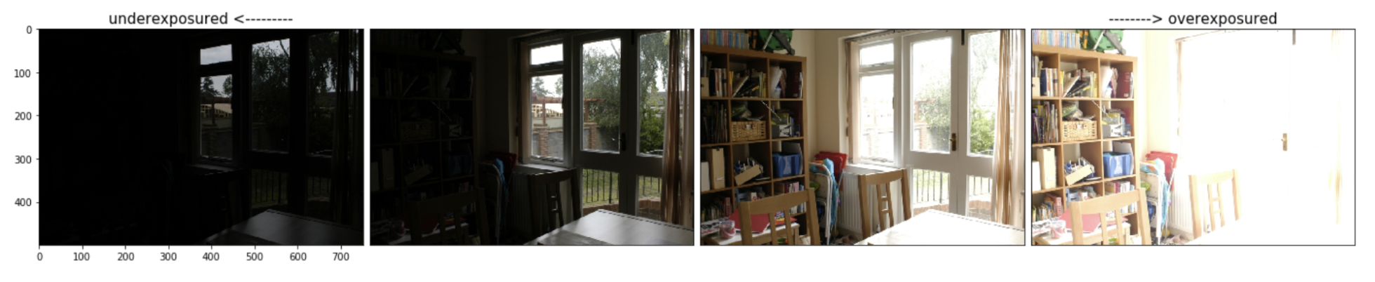
This picture shows the original images writh four different exposures, where an underexposed image becomes darker, but loses details in dark region. On the other hand, an overexposed image becomes brighter but loses details in bright region. The goal of the fusion is to obain an image with details over the entire region.

c. Construct weight maps

Three exponents for the weight maps are specified.

def getContrastWeight(self): return self.contrast_para
def getSaturationWeight(self): return self.sat_para
def getExposurednessWeight(self): return self.wexp_para

The following snippet constructs the weight maps. The dimension of weight map is identical to that of the original images (Width $\times$ Height $\times$ $N$), where $N$ is the number of images.

def ConstructWeightMap(self):
    self.contrast_para, self.sat_para, self.wexp_para = self.weightParam         
    self.W = np.ones((self.N, self.width,self.height),dtype=np.float32)
        
    if self.contrast_para > 0:
        self.W = np.power(np.multiply(self.W, self.contrast()),self.contrast_para)
            
    if self.sat_para > 0:
        self.W = np.power(np.multiply(self.W, self.saturation()),self.sat_para)
       
    if self.wexp_para > 0:
        self.W = np.power(np.multiply(self.W, self.well_exposedness()),self.wexp_para)    

    # normalize weight map, whose size will be (width,height,n_images)
    W_sum = self.W.sum(axis=0)
    self.W = np.divide(self.W, W_sum+1e-12)
    np.seterr(divide='ignore', invalid='ignore')        

According to eq.2, the weight maps are normalized, and the dimension of the weight map stack remains unchanged.

d. Failure of simple blending and alternative multiresolution blending using image pyramid

It turned out that the simple blending yielded a poor quality image with halos and seams.

\begin{equation} R_{ij} = \sum_{k=1}^N \hat{W}{ij,k} I{ij,k} \label{eq:5}
\end{equation}

Thus the authors considered an alternative method for blending using a Laplacian image pyramid.

A Laplacian image can be obtained by applying Laplacian operator given by the second derivatives of an intensity map $f=f(x,y)$

\begin{equation} Laplace(f) = \frac{\partial^2 f}{\partial x^2} + \frac{\partial^2 f}{\partial y^2} \label{eq:6} \end{equation}

This operator captures edges and texture on images.

An image pyramid is one kind of image processing technique to increase the image quality, which consists of downsized images from the original one. There is an original size image on the first level of the pyramid, and the size decreases by a quarter with each increase in the level.

The following picture shows the constructed 8-level Laplacian pyramid for one of the 4 original images.

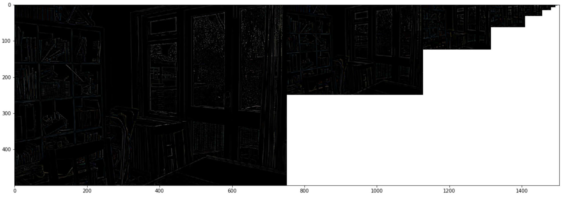
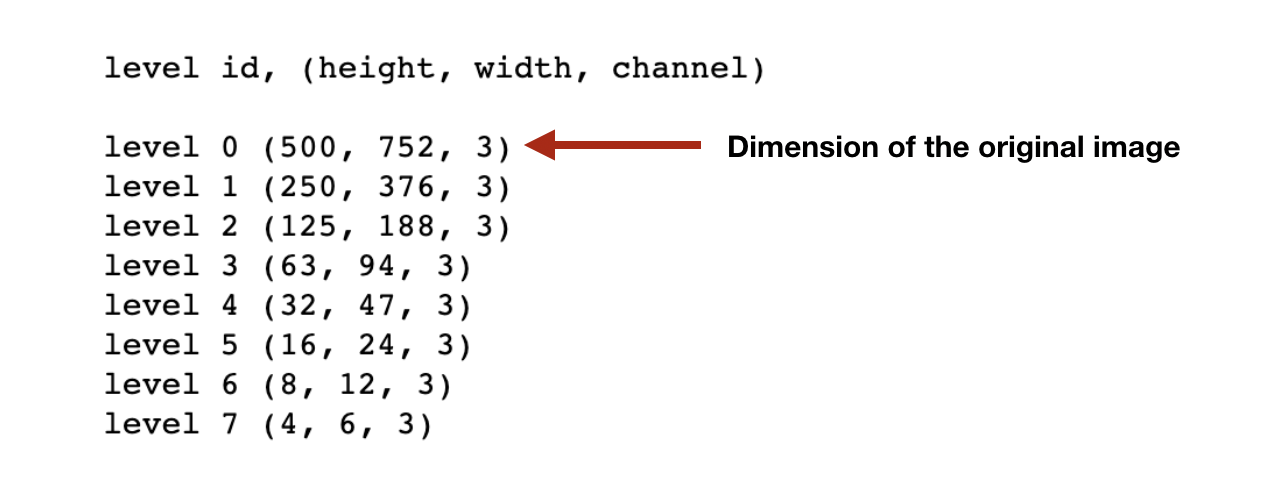
For our test image, the dimension of images on this pyramid changes as follows

This pyramid is the result of $\mathbf{L}[R]_{ij}^l$ in eq.3, where $l$ indicates a level on the pyramid.

e. Results

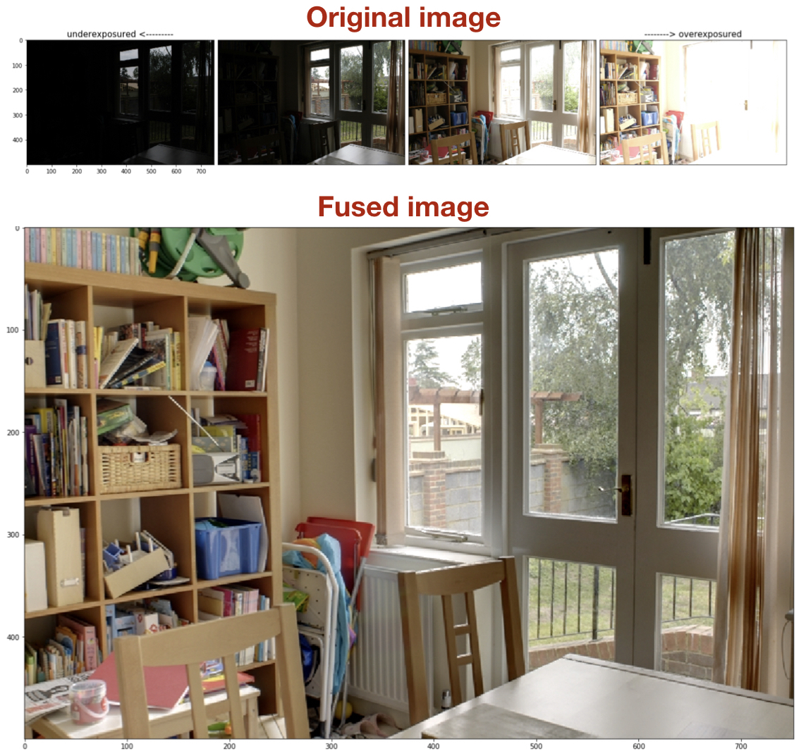
Using eq.4, the image is reconstructed, and the resulting image shows the great details on both inside and outside room. The combination of weight map exponents are $(\omega_C, \omega_S, \omega_E) = (1,1,1)$, by which the contrast, saturation, and exposedness are equaly constributed to the final image.

Wrapping it up

We have studied a multiresolution blending exposure fusion. The full implementation of the exposure fusion can be found here

Twitter Facebook LinkedIn

Voyager