Univariate Linear Regression (Numpy, tensorflow2.0, and Keras)

Univariate Linear Regression (ULR)

In this post, I study a Linear Regression(LR), which is a basic subject in Machine Learning (ML) algorithm. A single variable LR is considered. I will implement the LR with three different tools: Numpy, Tensorflow, and Keras, and their results will be compared to each other.

Hypothesis and loss function

• Hypothesis $y = w*x + b$ ($w$ for weight and $b$ for bias)

• Cost (loss) function is defined as a mean-squared error

  \begin{equation} J(w,b) = \frac{1}{2N}\sum_{i=1}^{N}\left( \hat{y}^{(i)} - y^{(i)} \right)^2 \label{eq:loss} \end{equation}

  where $\hat{y}^{(i)}$ is a predicted value for $i$th data point, and $N$ is the total number of data points The cost function is a quadratic function that would have a single global minima. The factor 2 in the cost function is a conventional introduction for the sake of simple calculation.

• The cost function is optimized by Gradient Descent The parameters w and b are updated as

  \begin{equation} w = w - \alpha \frac{\partial J}{\partial w}, \quad b = b - \alpha \frac{\partial J}{\partial b} \label{eq:w_updated} \end{equation}
  \begin{equation} \frac{\partial J}{\partial w} = \frac{1}{N}\sum_{i=1}^{N}\left(wx^{(i)}+b - y^{(i)} \right)x^{(i)} \label{eq:dJ_dw} \end{equation}
  \begin{equation} \frac{\partial J}{\partial b} = \frac{1}{N}\sum_{i=1}^{N}\left(wx^{(i)}+b - y^{(i)} \right) \label{eq:dJ_db}
  \end{equation}

Implementation

0. Module load and Data Acquisition

Loading modules

from sklearn.datasets import make_regression
import matplotlib.pyplot as plt
import numpy as np
import tensorflow as tf
import time

X, y = make_regression(n_samples=100, 
                       n_features=1, 
                       bias=10.0, noise=10.0, random_state=2)

where X is input data and y is a label data.

The dimemsion of label data is changed to (n_samples, 1).

y = np.expand_dims(y, axis=1)

Split the date into train and test sets with 80% and 20%, respectively.

train_x, train_y = X[:80], y[:80]
test_x, test_y   = X[80:], y[80:]

1. ULR with Numpy as from-scratch approach

The implementation in a class is as below

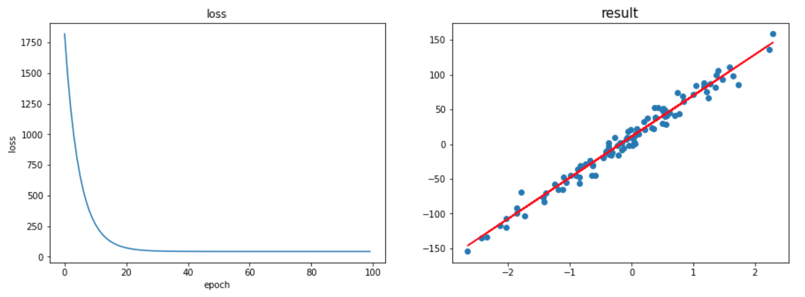
The result of the training is

2. ULR with Tensorflow 2.0

Next, we implement the ULR with the same dataset with tensorflow. Since the tensorflow is a software library, there are several functions to study. Besides, the LR is carried out in a batched data, which is much faster than training by individual data input.

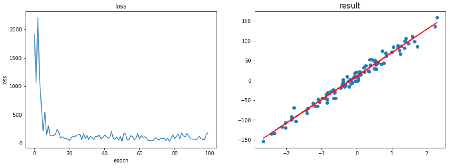
As shown in the result below, the batch train produces a noisy profile of loss function, which is eventually saturated at an optimized value. The result of train fits the data pretty well.

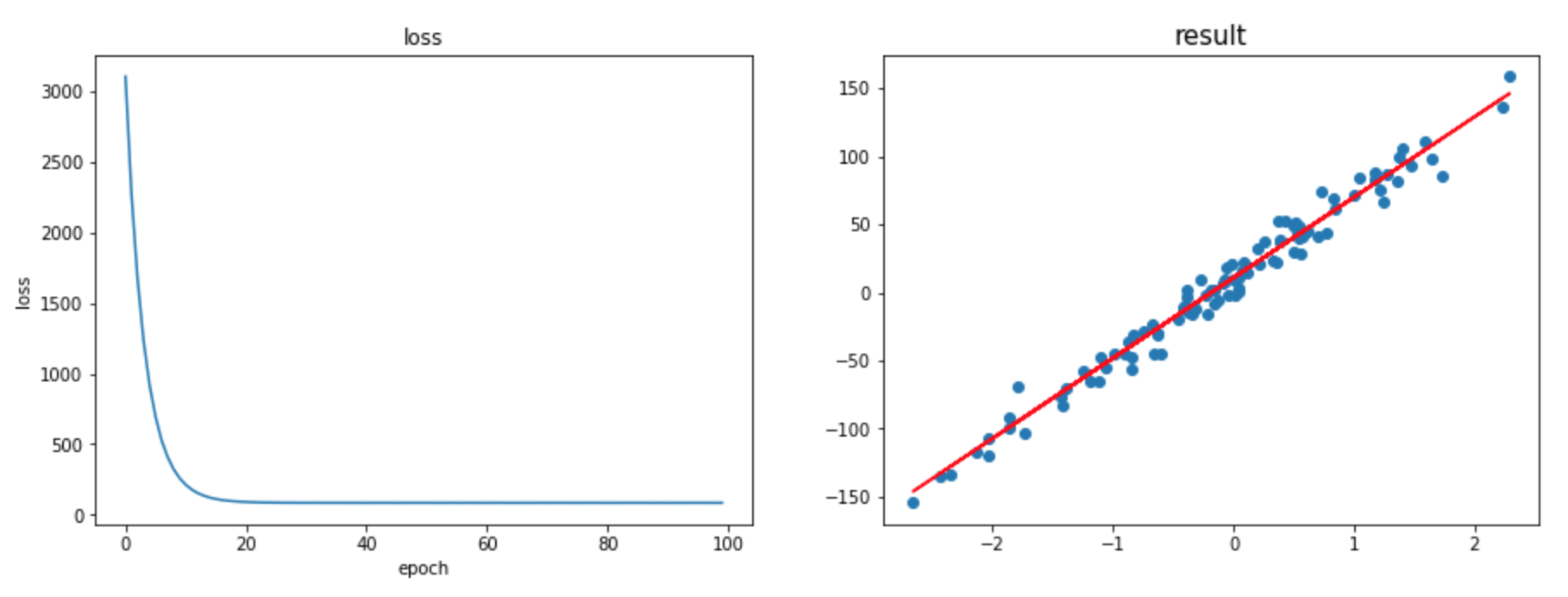
3. ULR with Keras

Concluding remarks

In this post, I have studied the Linear Regression of a single variable set (weight and bias). For complete study, I have implemented the Linear Regression with three different libraries: Numpy, Tensorflow 2.0, and Keras. This low- to high-level implementation provided a comprehensive understanding on how the algorithm works, which is especially very helpful for a beginner.

In the following post, as a continuation of self-study on ML, I will study a logistic regression.