Recovering HDR Radiance map by Camera Response Curves
Introduction
In this post, I will review and implement the Debevec’s algorithm for recovering HDR radiance map from photographs taken at different exposure times. This post is written as a series of study on exposure fusion to obtain a full detail image from differently exposed images. The implementation is made in Python using openCV.
What is High Dynamic Range(HDR)?
The Dynamic Range(DR) is defined as a ratio between darkest and brightest values. The High DR (HDR) refers then to an extended dynamic range of the brigthness. The brightness in the normal DR is ranged between 0 and 255 as 8-bit image, while the HDR extends such range to much larger than 255, up to $2^{16}-1 $ for 16-bit image. Thus, this extension allows to accommodate a high resolution of changes in the brighness, so that the HDR image captures great details in both bright and dark regions compared to DR images.
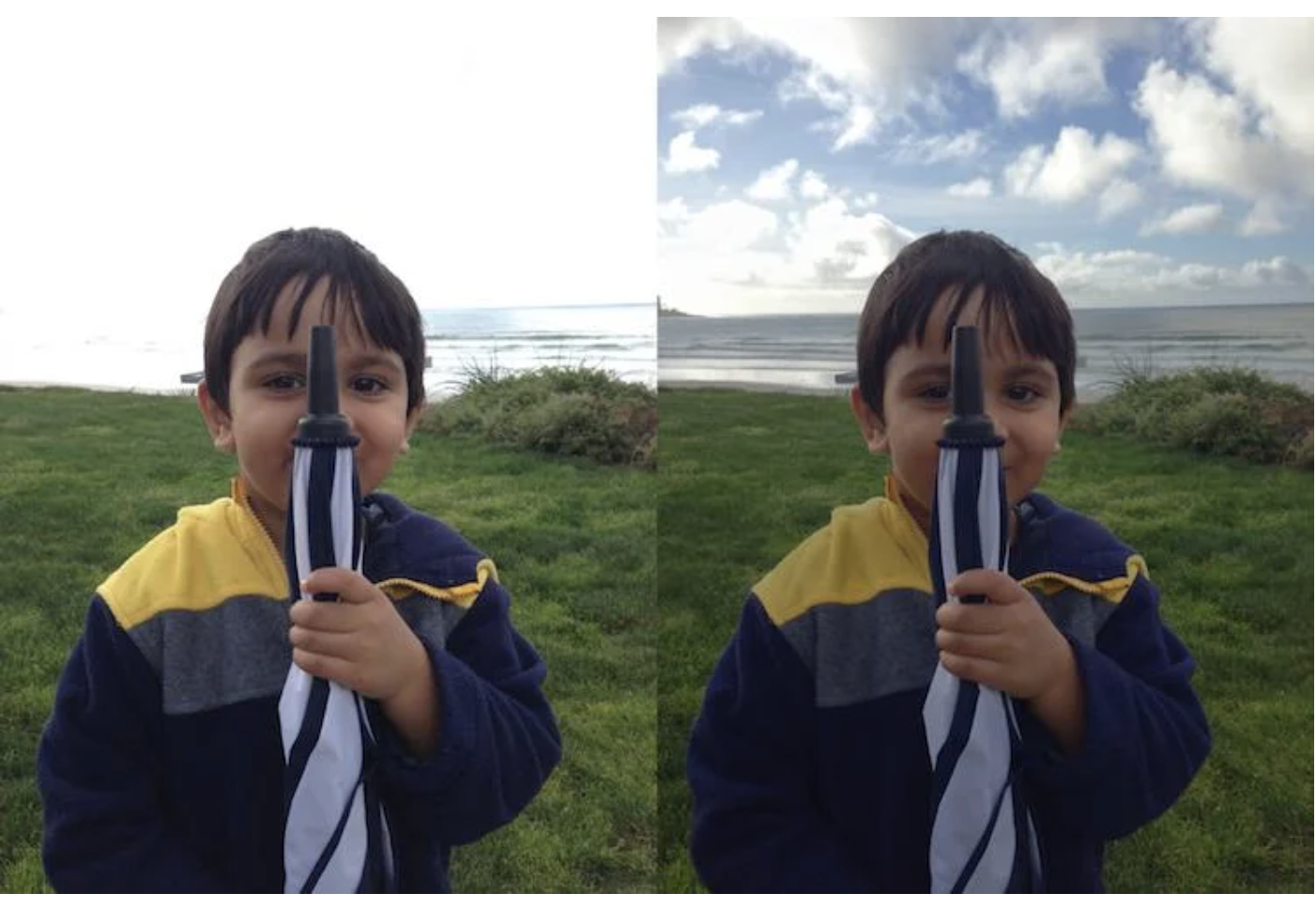
As shown in the two pictures above, the right one, which is HDR image, draws details in both the sky and the ground, corresponding to relatively bright and dark areas, respectively. On the other hand, in the left picture, the sky just appears as white background, which is due to limited dynamic range.
Recenlty, the HDR images have become very popular technique as they can be obtained at the level of software development.
Camera Response Function(CRF)
One very early attempt to produce an HDR image is to use a camera response curve, which relates the pixel values to irradiance of an object.
-
The film exposure is defined as $X = E \Delta t$, where $E$ is an irradiance at the film and $\Delta t$ is an exposure time, so $X$ is in unit of $J/m^2$. The exposure measures the total number of photons that each pixel absorb during the exposure time.
The assumption of this definition holds well in a reasonable range of the exposure times, but can break down under extreme conditions of very large or very low $\Delta t$.
-
the film reponse to variations in exposure $X$ is a non-linear function, called “characteristic curve” of the film, accounting for a non-linear relationship between pixel exposure $X$ and its intensity $Z$
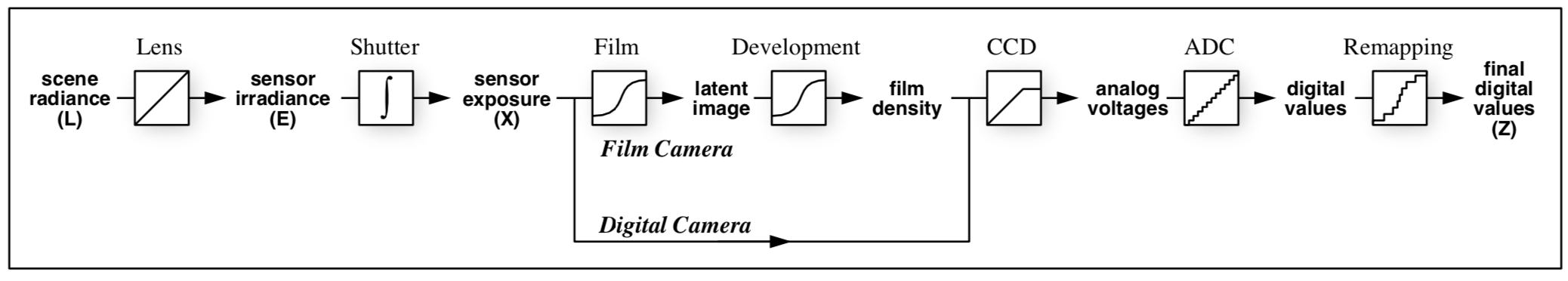
Image Acquisition Pipeline
There are many steps between scene radiance and final digital values. This figure shows how the scene radiance becomes pixel values. In the middle of the conversion, unknown mappings arise from exposure, development, scanning, digiziation, and remapping.
A nonlinear relation in the CRF includes an aggregate mapping from the scene radiancce to pixel values, made by several differently exposed images.
The main feature of Debevec’s algorithm is to find a nonlinear CRF for given images.
 The image is taken from ref.1.
Debevec’s Algorithm
The goal of this method is to render HDR cenes on conventional display devices, to be tested with real radiance maps as well as synthetically computed radiancce solutions
-
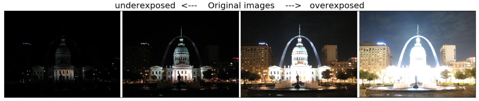
To cover the full dynamic range, one can take a series of photographs with different exposures, raising a question on how to combine these separate images into a composite radiance map
-
input: a number of digitized photographs taken from the same point with different exposure times (assumed that the scene is static and gathering these process is completed quickly enough so that the change in lighting can be safely ignored)
1. Camera Response Function
Suppose that we have a nonlinear function $f$ mapping the exposure $X$ to pixel values $Z$,
\begin{equation} f(X) = Z \longleftrightarrow X = f^{-1}(Z), \label{eq:exposure} \end{equation}
Then the reconstruction of the irradiance map from the pixel values can be obtained by applying inverse $f$, where $f$ is assumed to be a smooth and continuous function.
Eq.1 can be expressed with pixel($i$) and image($j$) indices as follow
\begin{equation} E_i \Delta t_{j} = f^{-1}(Z_{ij}) \label{eq:irradiance} \end{equation}
where $Z_{ij}$ indicates $i$th pixel values of $j$th image. This equation can be rewritten as follow
\begin{equation} g(Z_{ij}) = \ln E_i + \ln \Delta t_j \label{eq:log_g} \end{equation}
where $g = \ln f^{-1}$.
2. Weighted Objective Function for CRF Optimization
\begin{equation} O = \sum_{i=1}^{N}\sum_{j=1}^{P} \left( \omega(Z_{ij})\left[g(Z_{ij}) - \ln E_i - \ln \Delta t_j \right]\right)^2 + \ \lambda \sum_{z=Z_{min}+1}^{Z_{max}-1} \left[ \omega(z)g^{‘’}(z)\right]^2 \label{eq:obj_func} \end{equation}
The first term ensures that the solution satisfies eq.3 in a least square sense. The second term gives a smoothness, where the second derivative is given as a discrete form $g^{‘’}(z) = g(z-1) - 2g(z) + g(z+1)$ and $\lambda$ is a weight of the second term over the first one. $P$ and $N$ are the number of photographs and of pixels, respectively.
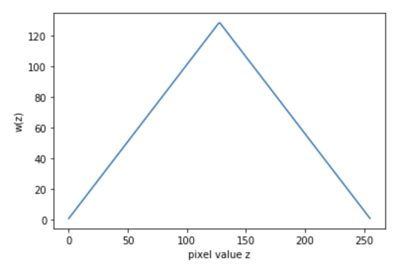
$\omega(z)$ is a weight function to impose the smoothness and fitting terms toward the middle of the response curve, which is chosen as a simple hat function as
\begin{equation} \omega(z) = \begin{cases} z-Z_{min}, & \text{for} \,z \leq \frac{1}{2}\left(Z_{min}+Z_{max}\right) \ Z_{max}-z, & \text{for}\, z > \frac{1}{2}\left(Z_{min}+Z_{max}\right) \end{cases} \label{eq:weight_func} \end{equation}
When measuring the response curve, the pixel locations should be chosen in a way that they are reasonably evenly distributed over $Z_{min}$ and $Z_{max}$, so that the pixels are to be well sampled from the images.
3. Constructing HDR Radiance Map
Once the response curves have been obtained, the original images can be merged into a single HDR image via
\begin{equation}
\ln E_{i} = \frac{\sum_{j=1}^{P}\omega(Z_{ij})\left(g(Z_{ij} - \ln \Delta t_{j}) \right) }{\sum_{j=1}^{P}\omega(Z_{ij})}
\label{eq:HDRmerge}
\end{equation}
Where, $P$ denotes the number of photographs, that is, the number of different exposure times. $Z_{ij}$ is the $i$th pixel’s value on $j$th image.
Combining the mutiple exposures has the effect of reducing noises. The picture below is the merged HDR map, which looks somewhat bright, this is because the sampling of bright pixels was made with an equal probability as dark parts.
Python Implemention
1. Load Images
Here, we considered four images taken with different exposure times, which are loaded with exposure times by the following lines
where ‘self’ comes from the extraction from class (see the full code)
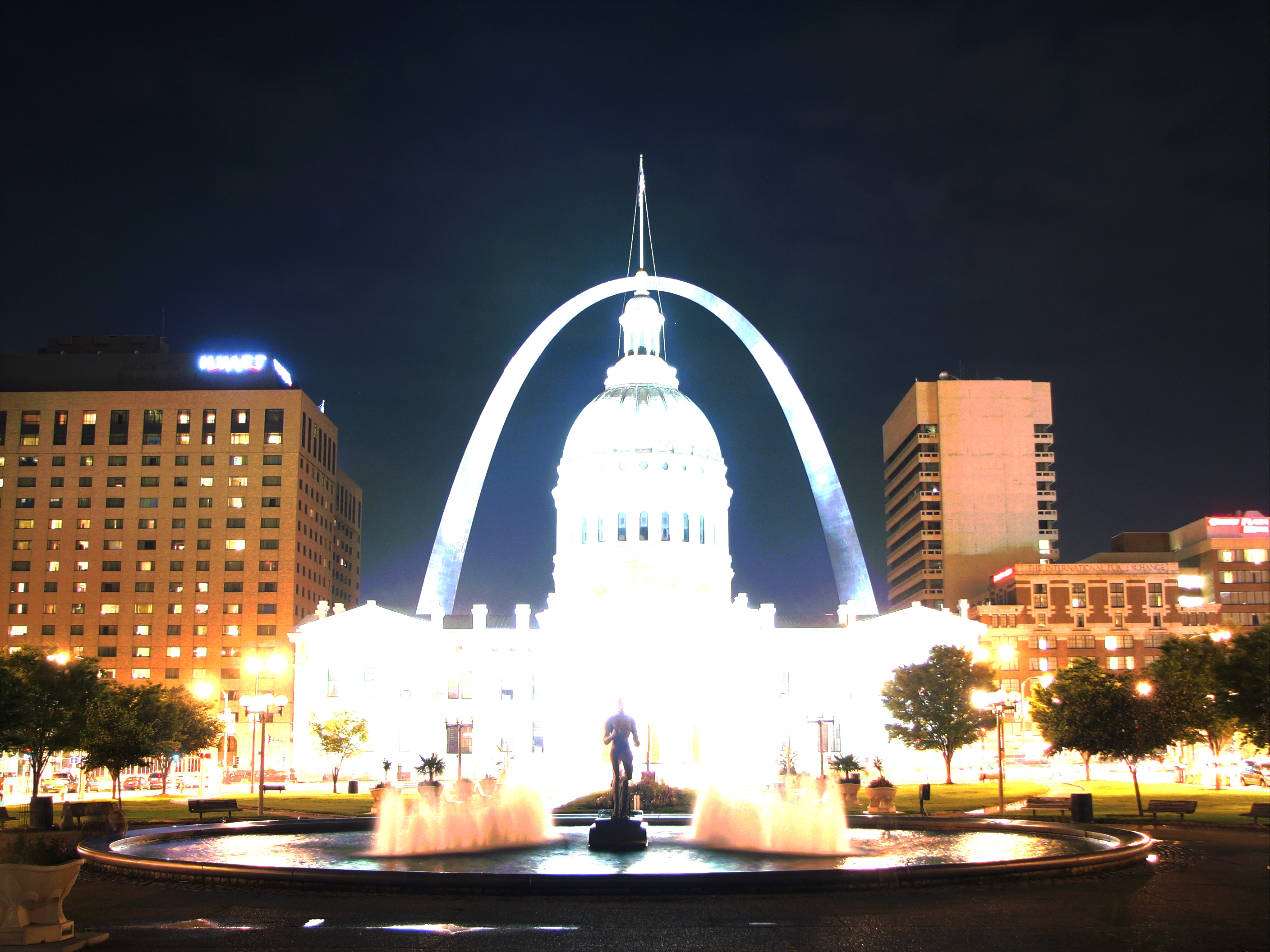
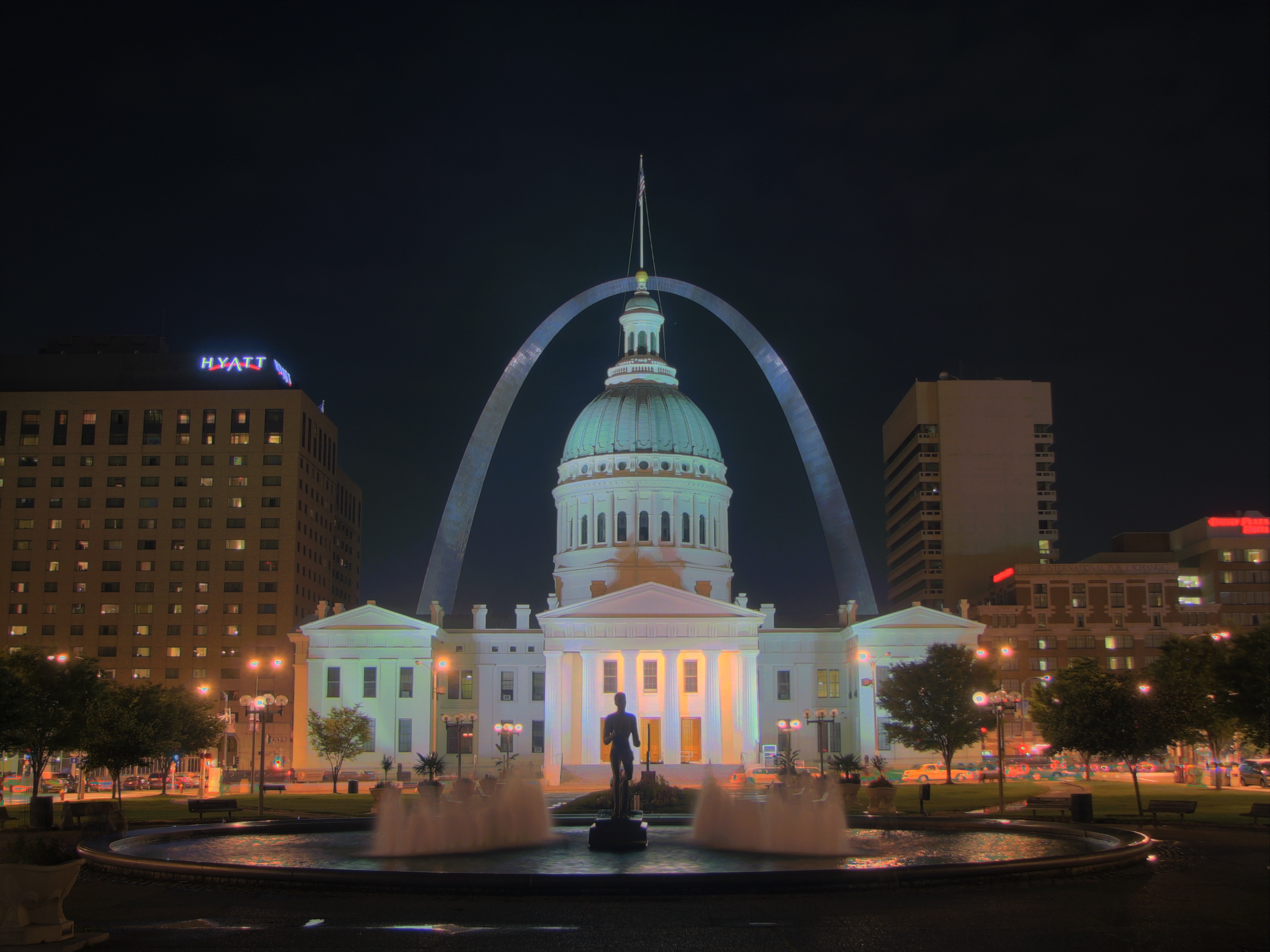
The loaded images appears as below
The exposure time increases from right to left.
The the above block contains also the declaration of variables associated with images, $N$ is the number of images, (here $N=4$), and row and col indicates the height and width of image in pixels. $l$ denotes $\lambda$ as a weighting factor for smoothness of the CRF.
Then, the images are aligned based on median threshold bitmap (MTB) method
The alignment of images is an important step, otherwise the fused image will get blurred.
2. Weight function
The weight function $\omega(z)$ in eq.5 is constructed as follow
The constructed weight function is shown as below, and this function will impose weight to the pixel values around the median of 255 in recovering HDR map.
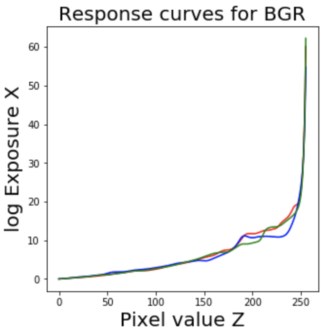
3. Camera Response Curves
A response curve is obtained by sampling pixels from given images. The number of samples is determined by $n_{sampling} (P-1) > (Z_{max} - Z_{min})$, which ensures a sufficiently overdetermined system as proposed in the original paper
This code block shows that we sampled pixels in an equal interval, and the pixel indices are stored in ‘sampleIndices’.
The following code shows that the sampling is made on individual channels.
Also, the exposure times are required to construct the response curve. In this procedure, the irrandiance $E$ is assumed to be 1, thus no contribution of $E$ to exposure $X$ is made as $\log E =0$.
Like many problems in computer vision, the problem of finding the CRF is set up as an optimization problem where the goal is to minimize an objective function consisting of a data term and a smoothness term. These problems usually reduce to a linear least squares problem which are solved using Singular Value Decomposition (SVD) that is part of all linear algebra packages. The details of the CRF recovery algorithm are in the original paper.
The picture below shows the constructed curves for three color channels
4. Merge images
The images are merged by eq.6, which yields a recovered fused radiance map as shown below.
This is an HDR image, which needs to be converted into a 24-bit image via tone mapping. Here, we used Drago’s method, where the parameters for Drago Tonemap are (gamma = 1, saturation=1, bias=0.85)
Wrapping it up
We have studied how to recover HDR radiance map from multiple exposure images. The full implementation of the exposure fusion can be found here.