Edge Enhancing (이미지 경계선 강화 필터링)
Introduction
In this post, we will study edge enhancement algorithms. There are several methods, most of which uses convolutions with a filter. Among them, we will look over three respresentative ones: Laplace operator, Difference of Gaussians, and Unsharp filter.
Python implementations can be found in the following links for each algorighms
1. Laplace Operator
2. Difference of Gaussians
3. Unsharp Filter
1. Laplace Operator
The Laplace operator takes second derivatives of an intensity map $f(x,y)$, where $x,y$ indicate a coordinate of pixels on the images.
\[\begin{eqnarray} \mathbf{L} &=& \nabla^2 f(x,y) \nonumber\\ &=& \left[\frac{\partial^2}{\partial x^2} + \frac{\partial^2}{\partial y^2} \right] f(x,y) \end{eqnarray}\]As shown below, for 1-D intensity profile, the Laplace operator captures the location at which the intensity changes most rapidly, which is surrounded by the opposite signs of intensity, enhancing edge.

However, the Laplacian filter is very sensitive to noise despite a better performancce on edge detection. This side effect is suppressed by applying Laplace operator to Gaussian blurred image that has already removed noise by blurring. This is called Laplacian of Gaussian(LoG).
\[\begin{eqnarray} \mathrm{LoG} &=& \nabla^2 G(x,y) \nonumber\\ &=& -\frac{1}{\pi \sigma^2}\left[ 1- \frac{x^2+y^2}{2\sigma^2} \right] \mathrm{e} ^{-\left(x^2+y^2\right)/2\sigma^2} \end{eqnarray}\]2. Difference of Gaussian (DoG)
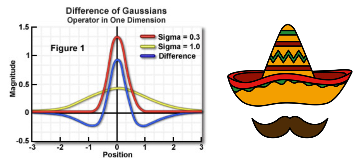
\[\begin{eqnarray} G_1(x,y) = \frac{1}{\sqrt{2\pi\sigma_1^2}}\exp\left(-(x^2+y^2)/2\sigma_{1}^2\right)\nonumber\\ G_2(x,y) = \frac{1}{\sqrt{2\pi\sigma_2^2}}\exp\left(-(x^2+y^2)/2\sigma_{2}^2\right) \end{eqnarray}\]These two Gaussian filter produces two blurred images. Difference of Gaussians is then made by subtracting more blurred image from less blurred one, ensuring that $\sigma_1 < \sigma_2$.
\begin{equation} f_{\mathrm{sharpened}}(x,y) = f(x,y)* G_1(x,y) - f(x,y) * G_2(x,y) \label{eq:conv} \end{equation}
where $* $ indicates convolution operator.
The DoG curve resembles a Mexican hat as shown below.

The resulting curve retains the location of maximum intensity, and surrounding of the location decreases to negative intensities in both sides, which makes the edge distinctive.
3. Unsharp Filter
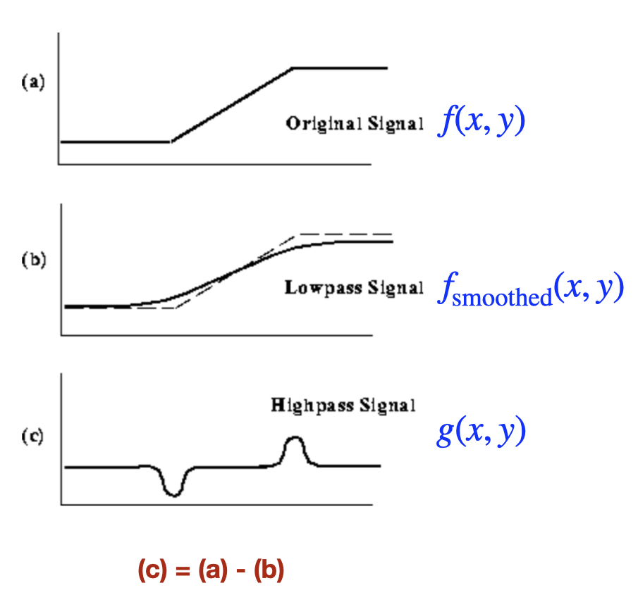
The unsharp filter is also used to enhance edges and other details on images. As one of spatial sharpening, the principle is pretty much similar to that of DoG, in a way that a smoothed image is subtracted from its original one, which produces a high-pass signal’s edge image.
\begin{equation} g(x,y) = f(x,y) - f_{\mathrm{smoothed}}(x,y) \label{eq:sub} \end{equation}
where $g(x,y)$ denotes the edge image.
A better understanding can be made in a signal pattern as shown below.
 |
|---|
| taken from Ref.3: The bottom panel (c) is obtained by subtracting (b) from (a). |
The resultant sharpened image can then be obtained by adding the edge image to the original one:
\begin{equation} f_{\mathrm{sharpened}}(x,y) = f(x,y) + kg(x,y) \label{eq:conv2} \end{equation}
where $k$ is a scaling constant, typically set from the range between 0.2 and 0.7. The sharpness of an image becomes enhanced as $k$ increases.
Wrapping up
We have studied three respresentative algorithms for edge enhancement: Laplace Operator, Difference of Gaussians, and Unsharp filter. Python implementations of these algorithms can be found in the links attached at the beginning of this post.
As a series of fundamental study of image processing algorithms, the following post will be covering image fusion and blending using image pyramid.